Lab Notebook
Laboratory Notebook Index
| Experiment Date | Title | ||
|---|---|---|---|
| 5/28/24 | Get a lightbulb to light | ||
| 5/29/24 | Series Circuits & Parallel Circuits | ||
| 5/29/24 | Use of an ammeter | ||
| 5/30/24 | Does current diminish as it flows? | ||
| 5/30/24 | Resistance | ||
| 5/31/24 | Potentiometer | ||
| 5/31/24 | Use of a voltmeter | ||
| 6/7/24 | Basic rules in Series Circuits & Parallel Circuits | ||
| 6/8/24 | Voltage, Current, Resistance | ||
| 6/9/24 | Measurement of an Unknown Resistance by Current-Voltage Method | ||
| 6/9/24 | Magnetic Field | ||
| 6/9/24 | Magnetic Effect of Electric Current | ||
| 6/14/24 | Electromagnet | ||
| 6/14/24 | Forces on Currents in Magnetic Fields |
Experiment 1: Get a lightbulb to light
Equipment: 1.5-V Battery (AA battery), one lightbulb, one wire
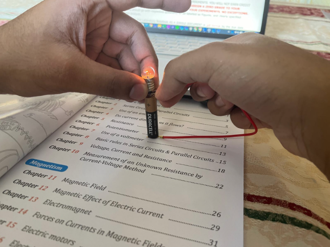 Figure 1
Data & Analytics: I knew that the electric current was flowing due to the fact that the positive terminal was connected to one end of the wire, and the negative terminal was connected to the other end of the wire. This led to the bulb lighting up, showcasing that the current was flowing. The lit bulb diagrams show a complete loop of wires, while the unlit bulb diagrams show a broken loop. As shown by Figure 1, this suggests that for the bulb to light up, there needs to be a complete loop for the electric current to flow through.
Conclusion: Any closed loop or conducting path allowing electric charges to flow is called an electric circuit. This experiment focused on the conditions that create current in an electric circuit, resulting in a product (light) being formed. It is possible to get the bulb to light with a battery, a lightbulb, and a wire. The battery supplied power, the lightbulb served as the output, and the wire facilitated electricity flow. This basic setup not only taught us about circuit fundamentals but also showcased their practical application in everyday devices. The conditions that create current in an electrical circuit involve having a closed loop or conducting path, enabling the flow of electric charges. This typically requires a power source (such as a battery), conductive materials (like wires), and a load (such as a lightbulb) that consumes the electrical energy, resulting in the formation of current within the circuit.
Experiment 2: Series Circuits & Parallel Circuits
Equipment: 1.5-V Battery (AA battery), two lightbulbs, two lightbulb sockets, some switches,, some wires
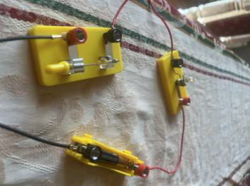 Figure 2
Data & Analytics: In Experiment A, a series circuit was constructed by connecting a lightbulb and a switch in a single path with a battery. The current flowed from the positive terminal of the battery, through the lightbulb, through the switch, and back to the negative terminal of the battery. As evidenced by Figure 2, when the switch was turned on, the circuit was complete, allowing current to flow and lighting up the bulb. Turning the switch off broke the circuit, stopping the current flow and causing the lightbulb to turn off. In Experiment B, a parallel circuit was formed by connecting two lightbulbs and two switches such that each lightbulb had its own independent path to the battery. The current flows from the battery through either Lightbulb A or Lightbulb B, depending on the state of their respective switches. When Switch A was on, Lightbulb A lit up, and when Switch B was on, Lightbulb B lit up. If both switches were on, both lightbulbs lit up, and if both switches were off, neither lightbulb lit up. This setup demonstrated the characteristics of a parallel circuit, where each branch operates independently, allowing each lightbulb to be controlled separately by its switch.
Conclusion: A series circuit refers to a current where all the current flows through each device sequentially. In this setup, if the circuit becomes open due to the switch being turned off or the lightbulb’s filament burning out, disrupting the connection, the flow of current ceases entirely. Conversely, a parallel circuit involves multiple current paths. The current from the power supply splits and flows through both lightbulbs simultaneously. When switch B is turned off in the parallel circuit, the flow of current through lightbulb B is halted, resulting in the non-operation of lightbulb B. Experiment A illustrated a series circuit, where components were connected sequentially, and current flowed through each device in a single path. When the switch was turned on, completing the circuit, the lightbulb illuminated, but when switched off, the flow of current ceased, and the lightbulb turned off. In contrast, Experiment B showcased a parallel circuit, where multiple current paths were established, allowing each lightbulb to operate independently.
Experiment 3: Use of an ammeter
Equipment: 1.5-V Battery (AA battery), one lightbulb, one switch, one ammeter, one lightbulb socket, some wires
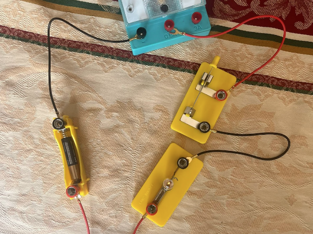 Figure 3
Data & Analytics: When connecting the 0.6A terminal, the smallest scale that can be obtained is -1. When connecting the 3A terminal, the smallest scale that can be obtained is 0. The readings for Experiment A are 1 & 0, and for Experiment B are -1 & 0. The current in both experiments are different due to the placement of the battery. I would most likely use the 0.6A range, as it allowed for more variation for the data.
Conclusion: To measure the current in an electric circuit using an ammeter, one must first ensure that the ammeter is properly connected in series with the component whose current is to be measured. This means that the current flowing through the circuit must pass through the ammeter. Begin by turning off the power supply to the circuit and selecting the appropriate current range on the ammeter to avoid damaging the device. Connect the positive lead of the ammeter to the positive side of the power source or component and the negative lead to the negative side, ensuring secure and correct connections.
Once the ammeter is connected and the power supply is turned on, observe the needle or digital display on the ammeter. To read the current on an analog ammeter, note the position of the needle on the scale. Each mark on the scale represents a specific value, depending on the range selected. If the needle points between two marks, interpolate to estimate the current. For a digital ammeter, simply read the numerical value displayed. Always double-check the range setting to ensure that the reading corresponds accurately to the current range selected. Properly interpreting these readings is crucial for accurately assessing the current flowing through the circuit, allowing for precise measurements and analysis.
When connecting the 0.6A terminal, the smallest scale that can be obtained is -1. When connecting the 3A terminal, the smallest scale that can be obtained is 0. The readings for Experiment A are 1 and 0, and for Experiment B are -1 and 0. The current in both experiments differs due to the placement of the battery. I would most likely use the 0.6A range, as it allowed for more variation in the data.
Experiment 4: Does current diminish as it flows?
Equipment: 1.5-V Battery (AA battery), two lightbulbs, some wires, one switch, two light sockets, one ammeter
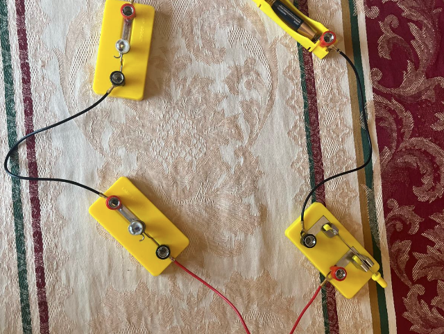 Figure 4
Data & Analytics: The current between the lightbulbs will be the same as the current before the lightbulbs. In a series circuit, the current is consistent throughout because there is only one path for the current to flow. This is confirmed in Figure 4, as it is clear that the brightness of the lightbulb are the same. That means the same amount of charge is present.
Conclusion: In a series circuit, the current remains consistent throughout the entire circuit. This means that if the lightbulbs are identical, they will have the same brightness because the same current flows through each bulb. Whether measured before, between, or after the lightbulbs, the current will be identical at all points. Consequently, the current does not decrease as it passes through different elements in the circuit. This uniformity ensures that identical lightbulbs will shine with equal brightness, as they all receive the same current.
Experiment 5: Resistance
Equipment: 1.5-V Battery (AA battery), one lightbulb, some wires, one switch, one light socket, one ammeter, 5-Ω resistor, 10-Ω resistor
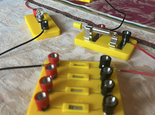 Figure 5
Data & Analytics: Through pure prediction, the lightness of the lightbulb in step 2 would most likely be more than the lightness of the lightbulb in step 3, as it is going from a 5-Ω symbol from a 10-Ω symbol, meaning that there is more resistance. This is confirmed in the trial of this using the system displayed in figure 5. This is demonstrated further, where using 5-Ω gives -0.2A, while using 10-Ω gives -0.1A, cutting it in half.
Conclusion: Resistance is a measure of how much a material opposes the flow of electric current. High resistance means that the material significantly impedes the flow of current, while low resistance indicates that the material allows current to flow more easily. When resistance increases, the current decreases if the voltage remains constant. This is because the opposition to the flow of electrons is higher, making it harder for the current to pass through. When resistance decreases, the current increases if the voltage remains constant. Lower resistance means less opposition to the flow of electrons, allowing more current to pass through. In summary, resistance opposes the flow of current in a circuit. The higher the resistance, the lower the current for a given voltage. This is present in the data that the experiment demonstrated, as it proves that the higher the resistance, the more the current is “blocked.” Going from 5-Ω to 10-Ω cuts the amps of the current by 50%, as it is by a factor of two. This proves that (at this level) it is close or at a linear progression.
Experiment 6: Potentiometer
Equipment: Two batteries, one lightbulb, one switch, one potentiometer, one ammeter, some wires
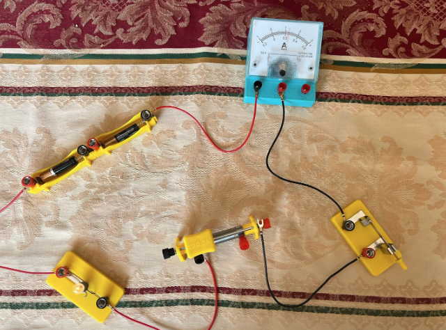 Figure 6
Data & Analytics: In the experiment, by moving the slider of the potentiometer from the left side to the right side, the charge decreased. As you move the potentiometer slide, the brightness of the lightbulb will change. The lightbulb will be dimmer when the resistance is higher and brighter when the resistance is lower. As noted in Figure 6, the slider is all the way to the left, which is when the lightbulb is the brightest. The current reading on the ammeter will decrease as the resistance increases (moving the slide one way) and increase as the resistance decreases (moving the slide the other way).
Conclusion: A potentiometer can be used to change currents in an electric circuit by varying the length of the metal wire, which in turn changes its resistance. A resistor is a device specifically designed to provide a certain amount of resistance. As shown in Figure 6, the slider on the potentiometer can adjust the resistance, impacting the illumination of the lightbulb. This is because a potentiometer acts as a variable resistor. By adjusting the potentiometer, you alter the circuit’s resistance, which affects the current flow. Different wiring configurations of the potentiometer will modify how resistance is adjusted, leading to varying brightness levels in the lightbulb and different readings on the ammeter. This experiment effectively demonstrates the interrelationship between resistance, current, and voltage in an electrical circuit.
Experiment 7: Use of a voltmeter
Equipment: Two batteries, one lightbulb, one switch one ammeter, several wires
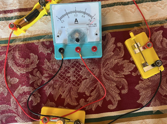 Figure 7
Data & Analytics: When using the 3A, the voltage goes to 1.6A, while when using the 0.6A, the voltage goes past 3A. By ensuring that the voltmeter is in parallel with the component whose voltage drop you are measuring, the voltmeter will show the voltage drop across the component on its display. The voltage in both experiments are not the same. To measure current, an ammeter must be connected in series with the component whose current you want to measure. This is because the current flows through the ammeter, allowing it to measure the flow of charge. To measure voltage, a voltmeter must be connected in parallel with the component across which the voltage drop is being measured. This configuration allows the voltmeter to measure the potential difference between two points.
Conclusion: To measure the current in an electric circuit, you must open the current path and insert an ammeter in series with the component whose current you want to measure. This allows the current to flow through the ammeter, enabling it to measure the flow of charge. In contrast, to measure the voltage across a component, you connect a voltmeter across the terminals of that component. The voltmeter, which has a very high resistance, is connected in parallel with the component. This high resistance ensures that the voltmeter does not draw significant current from the circuit, preventing any alteration in the voltage being measured. It is crucial to remember that an ammeter should never be connected in parallel because its low resistance could create a short circuit, potentially damaging the circuit or the ammeter itself. A short circuit occurs when there is a low-resistance connection between two points in an electric circuit, bypassing the intended path for the current. This can happen when the positive and negative terminals of a power supply are connected directly with a conductor of negligible resistance.
Experiment 8: Basic Rules in Series & Parallel Circuits
Equipment: Two 1.5-V batteries, one switch, one ammeter, some wires, one voltmeter, one 5-Ω resistor, one 10-Ω resistor
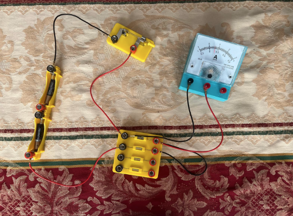 Figure 8
Data & Analytics: The relationship between V from V1 and V2 is that V1+V2 = V. The relationship between I1 and I2 is that I1 + I2 = I. The relationship from Experiment C showcases that V1 = V2 = V. In a series circuit, the total voltage drop across the series elements equals the sum of the voltage drops across each element, as V = IR. In a parallel circuit, the total current flowing from the battery equals the sum of the currents through each parallel branch. Each branch has its own current determined by its resistance and the applied voltage. In a parallel circuit, the voltage drop across each resistor is the same and equals the total voltage supplied by the battery.
Conclusion: In series circuits, the current is the same through all components. The total voltage drop is the sum of the individual voltage drops across each component. Because the same current flows through each part of a series circuit, I = I1 = I2 = I3, and V = V1 + V2 + V3. The relationship of current in a series circuit is equal to the potential difference of the source divided by the equal resistance. In parallel Circuits, the voltage drop across each parallel branch is the same. The total current is the sum of the currents through each branch. I = I1 + I2 + I3, and V = V1 = V2 = V3. The reciprocal of the equivalent resistance is equal to the sum of the reciprocals of the individual resistances.
Experiment 9: Basic Rules in Series & Parallel Circuits
Equipment: Three 1.5-V batteries, one ammeter, one voltmeter, one 5-Ω resistors, one 10-Ω resistor, one 20-Ω resistor, one potentiometer, one switch, some wires
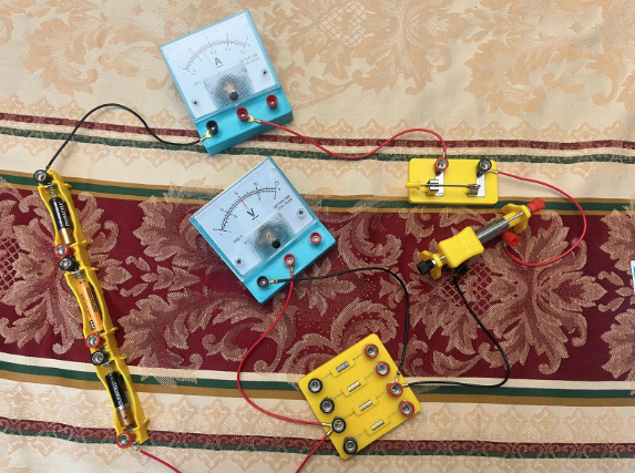 Figure 9
Data & Analytics: In Experiment A, the control variable was the resistance of the resistor, and in Experiment B, the voltage was the control variable.
Table 1: Trial
| Trial | I | V |
|---|---|---|
| 1 | 0 | 0.5 |
| 2 | 1 | 0.75 |
| 3 | 2 | 1 |
Table 2: Trial
| Trial | I | R | 1/R |
|---|---|---|---|
| 1 | 2 | 5 | 0.2 |
| 2 | 1 | 10 | 0.1 |
| 3 | 0 | 20 | 0 |
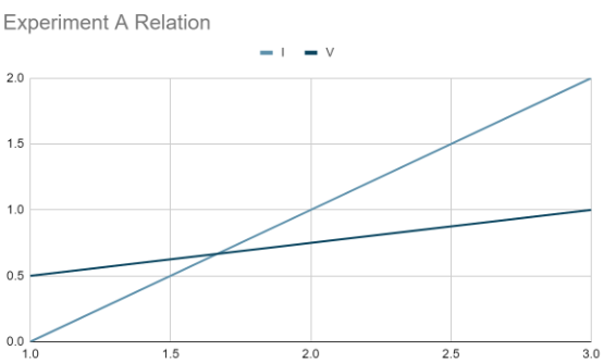
By keeping a consistent resistance with Experiment A, I was able to determine that increasing the I factor linearly affected the voltage. This relationship exists because increasing the electrical current would directly increase the voltage.
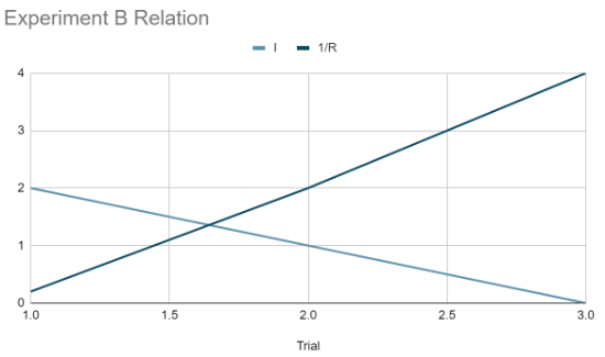
By keeping a consistent voltage with Experiment B, I was able to determine a relationship between I and 1/R, where decreasing I led to an increased 1/R, showcasing an inverse relationship between 1/R and I.
Conclusion: In this lab, we investigated the relationships between voltage, current, and resistance, confirming the fundamental principles of Ohm’s Law. In Experiment A, we varied the voltage across a constant resistance and observed that the current increased linearly with the voltage, indicating a direct proportionality between current and voltage. This was visually confirmed by plotting current versus voltage, which produced a straight line. In Experiment B, we examined the effect of varying resistance on the current for a fixed voltage. We found that the current decreased as the resistance increased, demonstrating an inverse relationship between current and resistance. Plotting current against the reciprocal of resistance resulted in a straight line, supporting the direct proportionality between current and the reciprocal of resistance. Combining these results, we derived Ohm’s Law. This formula succinctly describes how current is directly proportional to voltage and inversely proportional to resistance. Overall, the lab provided empirical evidence for Ohm’s Law, highlighting the importance of controlled variables and reinforcing our understanding of electrical circuit principles.
Experiment 10: Measurement of an Unknown Resistance by Current-Voltage Method
Equipment: Three 1.5-V batteries, one ammeter, one voltmeter, one unknown resistor, one potentiometer, one switch, some wires
 Figure 10
Data & Analytics: The factors that could have affected the result of the experiment include the temperature, the precision of measurement, and calibration of the ammeter and voltmeter. The need for lab data stems from averaging out random errors and the ability to detect anomalies. The potentiometer was included to adjust the current through the circuit, providing multiple data points. It also allows for more precise measurements.
| Trial | Current | Voltage | Resistance |
|---|---|---|---|
| 1 | 0.1 | 0.5 | 5 |
| 2 | 0.1 | 0.55 | 5.5 |
| 3 | 0.9 | 0.46 | 5.1 |
Conclusion: To measure an unknown resistance using the current-voltage method, we apply Ohm’s law, which states that R=V/I. In this method, we set up a circuit with a known current path including an ammeter, voltmeter, potentiometer, and the unknown resistor. By varying the potentiometer, we adjust the current and measure both the current (I) through and the voltage (V) across the unknown resistor. For each measurement, we calculate the resistance using the formula R=V/I. For instance, if we measure a current of 0.20 A and a voltage of 1.00 V, the resistance is R=1.00 V/ 0.20 A=5 Ω. Repeating this process for different current values still allows for an average value around 5. Multiple trials provide a reliable average resistance value, minimizing errors. Averaging the calculated resistances ensures accuracy, confirming that our unknown resistor is approximately 5 Ω. This method illustrates the practical application of Ohm’s law in determining resistance by directly measuring voltage and current.
Experiment 11: Magnetic Field
Equipment: One bar magnet, one horseshoe magnet, one compass, one iron fillings box
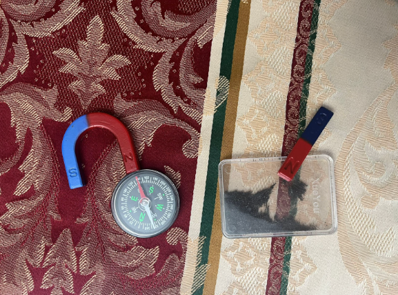 Figure 11
Data & Analytics: When placing the compass on a horizontal surface, the needle takes a moment to stabilize. Moving the north pole of a bar magnet towards the north pole of a horseshoe magnet results in repulsion, whereas moving it towards the south pole of the horseshoe magnet causes attraction. When an iron object is rubbed with the magnet and then brought near iron filaments, the filaments are attracted to the magnet. Placing the horseshoe magnet near the compass causes the red terminal (the north pole) to be attracted to the north side of the horseshoe magnet, and the white terminal to the south side. Like poles repel and opposite poles attract. The red terminal of the compass needle is the north pole, aligning with Earth’s magnetic north. The needle turns when its position changes to align with the magnetic field lines, indicating direction at that point.
Conclusion: This experiment demonstrates fundamental properties of magnets and magnetic fields. When placed on a horizontal surface, a compass needle requires time to stabilize due to the alignment process with Earth’s magnetic field. The interactions between the bar magnet and the horseshoe magnet reinforce the principle that like poles repel and opposite poles attract. This was evident when the north pole of the bar magnet repelled the north pole of the horseshoe magnet and attracted its south pole. Rubbing an iron object with a magnet and observing its effect on iron filaments illustrated that magnetic properties can be induced in certain materials. The response of the compass to the horseshoe magnet further highlighted the directional nature of magnetic fields, with the compass needle aligning itself along these invisible lines of force. The red terminal of the compass needle, representing the north pole, was attracted to the south pole of the horseshoe magnet, and vice versa. Overall, the experiment confirms that magnetic fields exert directional forces, causing aligned materials such as a compass needle to orient themselves along these fields. This behavior is due to the intrinsic properties of magnets, which have distinct north and south poles that interact predictably with each other and with induced magnetic materials. These observations are consistent with the fundamental principles of magnetism and provide a clear understanding of magnetic interactions and field alignment.
Experiment 12: Magnetic Effect of Electric Current
Equipment: Three 1.5-V batteries, one copper rod, one compass, one double rail module, one switch, some wires
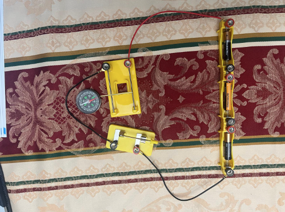 Figure 12
Data & Analytics: When the switch is closed and current flows through the copper rod, the compass needle deflects, indicating that the electric current produces a magnetic field around the rod. Upon opening the switch, the current stops, causing the magnetic field to disappear and the compass needle to return to its original position, aligned with the Earth’s magnetic field. Reversing the current direction results in the compass needle deflecting in the opposite direction, demonstrating that the magnetic field’s direction depends on the current’s direction.
Conclusion: The lab explores the magnetic effect of electric current, a fundamental concept in electromagnetism. By setting up a circuit with three 1.5-V batteries, a copper rod, a compass, and other components, the experiment demonstrates how electric current generates a magnetic field. When current flows through the copper rod, the nearby compass needle deflects, showing the presence of a magnetic field. This field disappears when the current stops, as observed when the switch is opened and the compass needle returns to its original position. Reversing the direction of the current causes the compass needle to deflect in the opposite direction, highlighting the dependency of the magnetic field direction on the current flow. The experiment underscores the relationship between electricity and magnetism, illustrating key principles that are essential in the functioning of devices like electromagnets and electric motors. Observing these effects helps in understanding the fundamental laws of electromagnetism and their applications in various technologies. It also emphasizes the importance of careful handling of electrical components to prevent overheating and ensure safety during experiments.
Experiment 13: Electromagnets
Equipment: Three 1.5-V batteries, one solenoid, one ammeter, one potentiometer, one switch, some wires, some paper clips
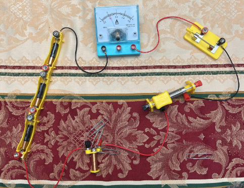 Figure 13
Data & Analytics: From the experiment, it is evident that the presence of an iron core inside the solenoid significantly enhances its magnetic field strength, as indicated by the increased number of paper clips attracted. The strength of the current flowing through the solenoid also directly impacts its magnetic field; higher currents result in stronger magnetic fields, attracting more paper clips, while lower currents produce weaker fields. Other factors that influence the magnetic field strength include the number of turns in the coil, with more turns creating a stronger field, and the material of the core, where materials with higher magnetic permeability, like iron, amplify the field. Additionally, the cross-sectional area of the coil affects the field strength, with larger areas accommodating more magnetic flux. The length of the solenoid also plays a role, as a shorter solenoid with the same number of turns will have a stronger magnetic field due to the denser packing of turns. Thus, the key factors impacting the strength of an electromagnet’s magnetic field are current strength, number of coil turns, core material, coil cross-sectional area, and solenoid length. Understanding these factors allows for the optimization of electromagnets for various applications by adjusting these parameters to achieve the desired magnetic field strength.
Conclusion: Conclusion: In this lab, we investigated the factors that affect the strength of an electromagnet’s magnetic field. By constructing a solenoid and measuring its ability to attract paper clips, we observed that an iron core significantly enhances the magnetic field strength. The strength of the current through the solenoid also directly impacts the magnetic field, with higher currents producing stronger fields. Additionally, we found that the number of turns in the coil, the material of the core, the coil’s cross-sectional area, and the solenoid’s length are crucial factors. More turns and materials with high magnetic permeability, like iron, increase the field strength. A larger cross-sectional area accommodates more magnetic flux, and a shorter solenoid with dense turns results in a stronger field. Understanding these factors allows for optimizing electromagnets for various applications. This experiment reinforced theoretical concepts and provided practical insights into manipulating and measuring magnetic fields, deepening our understanding of electromagnetism.
Experiment 14: Forces on Current in Magnetic Fields
Equipment: Three 1.5-V batteries, one double-rail module, one switch, one ammeter, one copper rod, one horseshoe magnet, one potentiometer, some wires
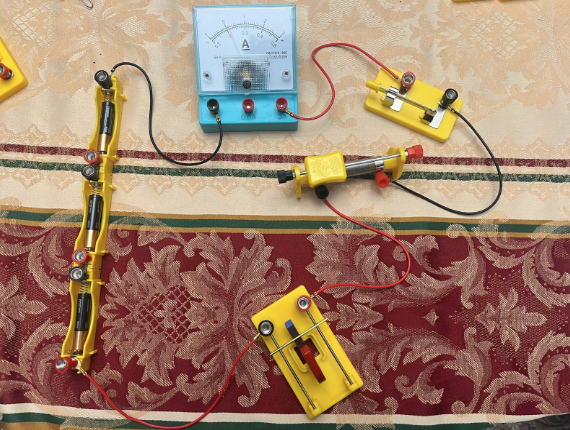 Figure 14
Data & Analytics: Before the current reached a certain strength, the copper rod remained stationary, but after the current reached a threshold strength, the rod experienced a force and moved. This occurs because a stronger current generates a larger magnetic field around the conductor, increasing the interaction with the magnetic field of the horseshoe magnet, resulting in a noticeable force on the rod. When the direction of the current was reversed, the direction of the force on the copper rod also reversed, consistent with the right-hand rule. Changing the direction of the magnetic field similarly reversed the direction of the force on the copper rod. This is because the force experienced by the conductor depends on both the direction of the current and the magnetic field, as described by the right-hand rule. The right-hand rule states that if you point your thumb in the direction of the current and your fingers in the direction of the magnetic field, the force exerted on the conductor will be in the direction your palm pushes. Therefore, reversing either the current or the magnetic field reverses the direction of the force. This experiment illustrates how electromagnetic forces act on current-carrying conductors within magnetic fields and emphasizes the practical application of the right-hand rule.
Conclusion: This experiment demonstrates the interaction between a current-carrying conductor and a magnetic field, a fundamental concept in electromagnetism. By placing a copper rod between the poles of a horseshoe magnet and passing a current through it, we observed that the rod experiences a force perpendicular to both the current and the magnetic field. This force causes the rod to move, and its direction can be predicted using the right-hand rule. Reversing the direction of the current or the magnetic field reverses the direction of the force, highlighting the vector nature of these quantities. The force increases with the current’s strength, indicating a proportional relationship. This experiment illustrates how electromagnetic forces are used in various applications, such as electric motors and generators. Understanding this principle is crucial for designing and operating devices that rely on electromagnetic interactions. The practical application of the right-hand rule provides a reliable method for predicting the behavior of current-carrying conductors in magnetic fields.